(Murad Banaji, 7th May 2020).
Germany provides some of the “cleanest” COVID-19 data from the point of view of exploring models of the pandemic. The first thing the German data demonstrates is that relatively simple, stochastic, agent-based modelling (code at https://github.com/muradbanaji/COVIDSIM, description at /research/modelling-the-covid-19-pandemic/), with most parameters fixed at their default values, can reproduce the data quite well (Figures 1 and 2 below). The parameters left at their default values include the average time from infection to death or recovery, and the beginning and end of infectivity. The main parameters which generally need to be altered to fit data from different outbreaks are: R0 (the basic reproduction number); the percentages of infected individuals quarantined and/or tested; the average date of quarantining; and parameters associated with mitigation, such as the degree of physical distancing, when it starts, and the extent to which restrictions on movement affect the total “infectible” population.
A specific point that the German data can be used to demonstrate is that we cannot use measured infection and fatality data to infer a fatality rate. Rather, we can vary an assumed fatality rate and see what this tells us about the total pool of infection. This is done in Figure 1 below.
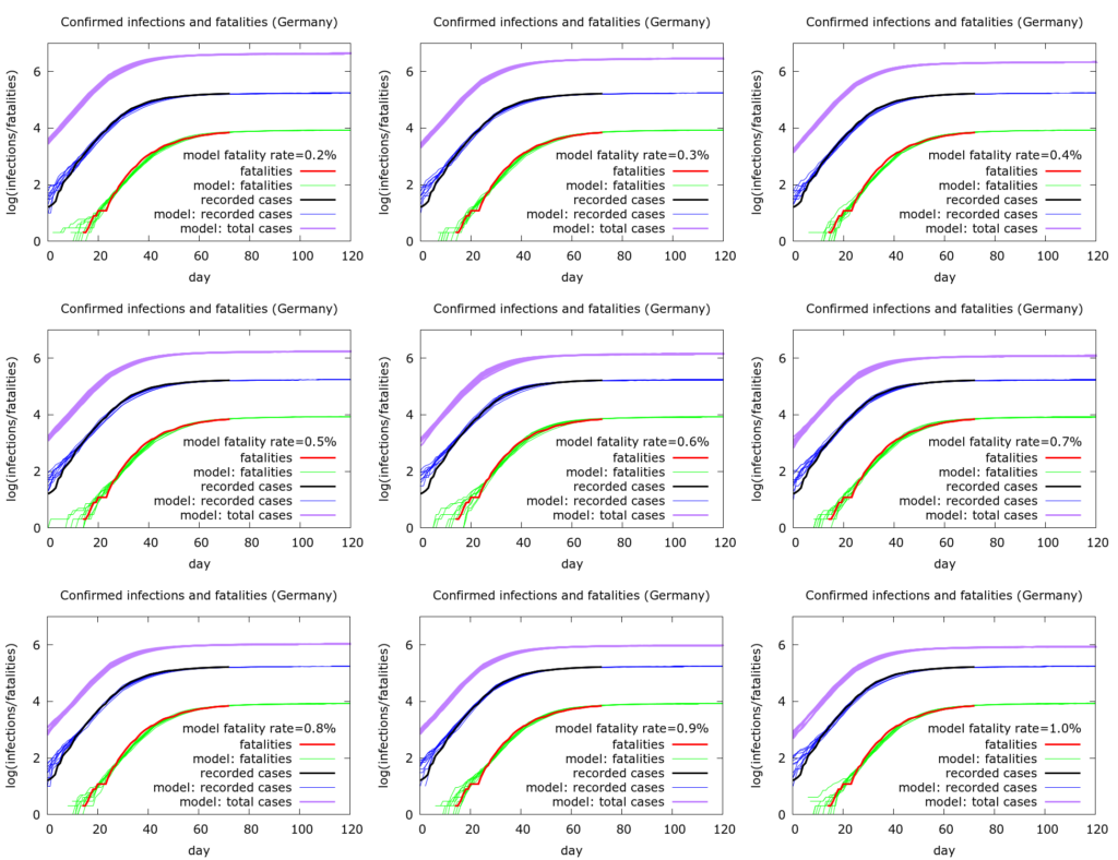
Figure 1. Nine simulations where we increase the fatality rate in the model from 0.2% to 1% and are still able to reproduce the observed testing and fatality data reasonably well. The estimated total infections, however, change in inverse proportion to the fatality rate, ranging (on May 7th) from about 800,000 (1% fatality rate) to 4 million (0.2% fatality rate).
All nine sets of simulations in Figure 1 (each set has ten simulations) fit the German data well. However the fatality rate changes from 0.2% to 1.0% as we move through the simulations. By rescaling three other quantities in the model – the percentage of individuals tested, the infectible population post-lockdown, and the rate of leak into this population – we get essentially the same dynamics with the different fatality rates. The model output that changes, however, is the total number of infections (purple curves). For completeness the exact values of model parameters used are given later.
So, for example, with a fatality rate of 1.0%, total current infections (as of May 7th 2020) number about 800,000, roughly five times recorded infections. In this scenario only about 1% of the German population has so far been infected, and testing is picking up about 20% of infections. At the other end of the spectrum, with a fatality rate of 0.2%, total infections number about 4 million, namely about 25 times recorded infections. In this scenario, about 5% of the German population has been infected, and testing is picking up only 4% of infections or so. Note that in none of these scenarios is there sufficient herd immunity to slow the pandemic nationally, although the picture might be different locally. For a significant degree of herd immunity to have developed nationally, the fatality rate would have to be exceedingly low – below 0.1%.
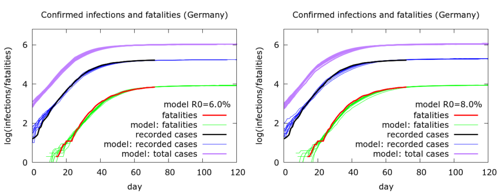
The next observation to make is that there is considerable over-parameterisation of the model (as one would expect). Apart from fatality rate, it is possible to change a variety of other parameters and still fit the data. So, for example, in Figure 2 the fatality rate is fixed at 0.8%, but other parameters are changed between the first and the second sets of simulations. In particular, R0 is increased from 6.0 to 8.0, but we can still fit the data reasonably well by altering quarantining (or self-isolation) levels, and the timing of lockdown: on the left 25% of people are quarantined and “lockdown” begins at the 30th death (~20th March); on the right, 50% of people are quarantined, and lockdown begins at the 10th death (~15th March). In reality there were an increasing number of measures being implemented around this period. Both sets of simulations agree, however, that testing is picking up about 16% of infections: as one would expect, this value depends primarily on the fatality rate.
All the simulations here project that the German outbreak continues to stabilise with deaths reaching between 8300 and 9000 by late June. These numbers assume, of course, that there is no let up in mitigation measures and consequent acceleration of spread.
To conclude, the model is able to fit the German data quite well, and with a variety of parameter values. Model predictions about total infection rate depend on the fatality rate (total infections equal, roughly 800,000 divided by the fatality rate as a percentage). The thing which most stands out in the German data is, naturally, the relatively high percentage of infections picked up by testing. The details of this percentage depend on the fatality rate; but at any given fatality rate we find that Germany is picking up 3-4 times the proportion of infections that the UK is doing. In most scenarios, this has actually been a key tool in control of the epidemic in Germany.
Appendix
For completeness here are the parameter values used to generate the 9 plots in Fig. 1 and the two plots in Figure 2. Note that a scaling was applied to speed up computations – all populations appear at one tenth of their value, and death rates are multiplied by 10.
Figure 1 (lexicographically ordered)
number_of_runs 10
death_rate 2.0, 3.0, 4.0, 5.0, 6.0, 7.0, 8.0, 9.0, 10.0
geometric 1
R0 6.0
totdays 150
population 8300000
inf_start 3
inf_end 14
time_to_death 17
dist_on_death 0
time_to_recovery 20
dist_on_recovery 0
initial_infections 10
herd 1
percentage_quarantined 25
percentage_tested 16.25, 24.375, 32.5, 40.625, 48.75, 56.875, 65, 73.125, 81.25
testdate 5
dist_on_testdate 0
haslockdown 1
lockdth 30
lockdownlen 150
infectible_proportion 0.048, 0.032, 0.024, 0.0192, 0.016, 0.0137, 0.012, 0.0107, 0.0096
pdeff_lockdown 50
popleak 4000, 2667, 2000, 1600, 1333, 1143, 1000, 889, 800
popleak_start_day 15
physical_distancing 1
pd_at_test 200
pdeff1 25
Figure 2:
number_of_runs 10
death_rate 8.0
geometric 1
R0 6.0, 8.0
totdays 150
population 8300000
inf_start 3
inf_end 14
time_to_death 17
dist_on_death 0
time_to_recovery 20
dist_on_recovery 0
initial_infections 10
herd 1
percentage_quarantined 25,50
percentage_tested 65,35
testdate 5
dist_on_testdate 0
haslockdown 1
lockdth 30,10
lockdownlen 150
infectible_proportion 0.0120
pdeff_lockdown 50
popleak 1000
popleak_start_day 15
physical_distancing 1
pd_at_test 200
pdeff1 25