(Murad Banaji 02/07/2020)
All data is taken from https://www.covid19india.org/. We refer to the period upto April 10th as the “early period”, and case and fatality data upto April 10th as “early data”. We assume that in the early days of the epidemic, all COVID-19 deaths were being accurately recorded. By April 10th there had been 7600 COVID-19 cases and 252 recorded COVID-19 deaths. Using April 10th as a cut-off date gives us a reasonable volume of data to work with while, at the same time, avoiding the latter half of April when the signature of missing deaths appears clearly in the data (see below).
We use the early data to work out a delayed case fatality rate (CFR) for a range of possible values of case-fatality reporting delay (C-F delay), the average delay between the time after infection when cases are recorded, and the time after infection when deaths are recorded. Assuming constant case detection, namely that these delayed values of CFR remain constant, allows us to estimate fatalities at any later point.
The approach, by example. To see how this process works consider, for example, a C-F delay of 8 days. (This would be obtained if, for example cases are typically recorded 13 days after infection, while fatalities are typically recorded 21 days after infection.) We’ll refer to the C-F delay under an assumed delay of d days as CFR_d. We want to estimate CFR_8. To do this we take a block of early fatality data and divide by a block of case data from 8 days previously to get a point estimate for CFR_8. We then take the geometric mean of several such estimates of CFR_8 to get a more robust estimate. In practice, we take 6-day blocks of data so that fatality numbers in each block are not too small, and do 12 such calculations as this seems to be about as many as we can manage before even the blocked fatality numbers get too small to be reliable. We obtain an estimate of CFR_8=0.116, i.e., 11.6%, (10.9%,12.5%). The numbers in brackets are a 95% confidence interval.
This tells us that fatalities today should be approximately 11.6% of cases 8 days ago. To estimate fatalities by April 30th, we just take cumulative cases 8 days earlier (April 22nd, when there were 21,372 cases) and multiply by CFR_8 to get 2484 (2319, 2662) fatalities. As only 1154 fatalities had been recorded by April 30th, this corresponds to fatality undercounting of about 54% (50%, 57%). Of course, the underlying assumption in this calculation is that case detection, the C-F delay, and IFR, all remained constant from the early period to the end of April. Note that although IFR was assumed to have remained constant, a value for IFR was not explicitly needed in this calculation.
To estimate infections we need two additional numbers: IFR and a typical delay between infection and when death is recorded, which we’ll term the infection-fatality delay, or I-F delay for short. To continue with the example above, let’s assume an IFR of 0.5% and an I-F delay of 21 days (in addition to the previously assumed C-F delay of 8 days). We can take the IFR and divide by CFR_8 to get a case detection rate at a delay of 8 days and assuming an IFR of 0.5%, of 0.043, i.e., 4.3% (4.0%, 4.6%). To estimate, say, infections by April 30th we look at total cases (21-8)=13 days later – i.e., on May 13th – and multiply by 0.043. This gives an estimated total of 1.82 million (1.69M, 1.94M) infections on April 30th. Reducing the I-F delay to, say, 18 days reduces naturally reduces such prevalence estimates – in this case by about 15%.
Estimates of delayed case fatality rates and missing fatalities at the end of June. Here are the values of CFR_d to 3 s.f. estimated from early data for d = 0, …, 12 respectively: 3.26%, 3.79%, 4.39%, 5.11%, 6.02%, 7.06%, 8.35%, 9.82%, 11.6%, 13.8%, 16.4%, 19.7% and 23.6%. Estimated fatalities on a given day can be calculated by multiplying CFR_d by cases from d days earlier. Using these numbers we get estimates for fatalities on June 29th for d = 0, …, 12 as: 18492, 20833, 23263, 26022, 29572, 33412, 38065, 43256, 49634, 56623, 65098, 75162, and 86780. There were 16,904 recorded fatalities on June 29th, so undercounting ranges from 8.6% (at d=0) to 80.5% (at d=12).
Estimates of prevalence on June 8th. Assuming an IFR of 0.5% and an I-F delay of 21 days we get the following estimates for cumulative infections on June 8th for d = 0, …, 12 respectively (in millions, to 3 s.f.): 3.70, 4.17, 4.65, 5.20, 5.91, 6.68, 7.61, 8.65, 9.93, 11.3, 13.0, 15.0, 17.4.
The narrative of missing deaths over time. Note that the estimates for missing COVID-19 deaths rely only on the C-F delay, but not on the IFR or the I-F delay. What is remarkable is the rapid progression in undercounting these techniques suggest occurred during the second half of April. This is best seen in the figure below. We see that for all values of C-F delay between 2 days and 10 days, there is a rapid increase in the percentage of deaths which are going “missing” during April. The increase is most rapid for higher values of C-F delay, but clear at all the values.
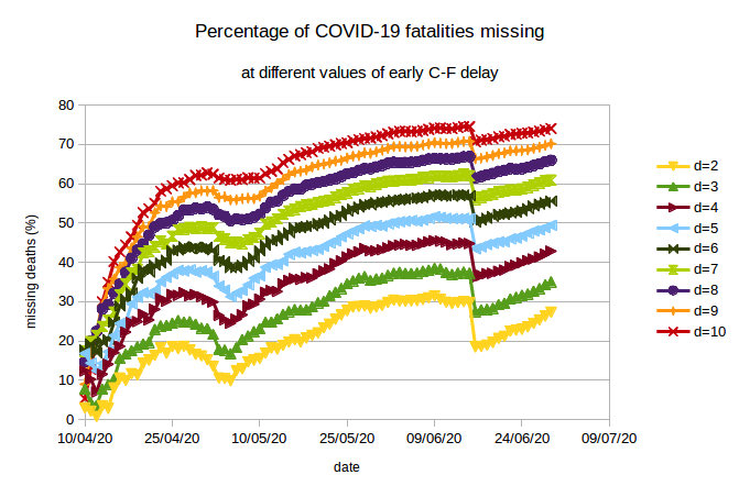
The rapid increase in missing deaths in April is followed by a “correction” during early May when, for example, West Bengal added into its count a number of COVID-19 fatalities which had previously been omitted. But the rise began again after this, and continued until another correction in mid-June when Maharashtra added a number of missing fatalities into its count. The rise has continued again subsequently, indicating that despite the corrections fatality undercounting has not slowed.
Explanation for missing fatalities. Note that a large number of missing COVID-19 deaths is an inescapable conclusion of analysis based on the early data, and that this conclusion does not rely on assumptions about IFR. Several previous modelling studies have also pointed to missing COVID-19 fatalities. But “missing deaths” could also be interpreted as a drop in IFR – the deaths are “missing” because they did not occur. So, is it possible that IFR actually dropped significantly rather than fatalities being unrecorded?
The large increase in missing fatalities in April itself, alongside the narrative evidence of fatality undercounting from several states, as discussed here, make this implausible. This is not to say that other possible causes, including the spread of disease in a younger population, or more effective treatment should be dismissed; but they should not be accepted without further evidence. In my view the most likely cause of the major part of the apparent drop in IFR is that fatalities are not being registered/recorded.
I would speculate that the reason for missing fatalities is a combination of misclassification of COVID-19 deaths of people with comorbidities, poor recording of data, data not being correctly shared between different bodies (hospitals, different levels of government), suspected COVID-19 fatalities not being tested (for political reasons or perhaps because of a shortage of kits), and more and more deaths occurring at home or in nursing homes.
Estimating the C-F delay in the early period. The claim of significant death undercounting is robust over a range of values of C-F delay, but the extent of undercounting varies significantly depending on the presumed C-F delay. The question then arises of whether it is possible to estimate the C-F delay using early data.
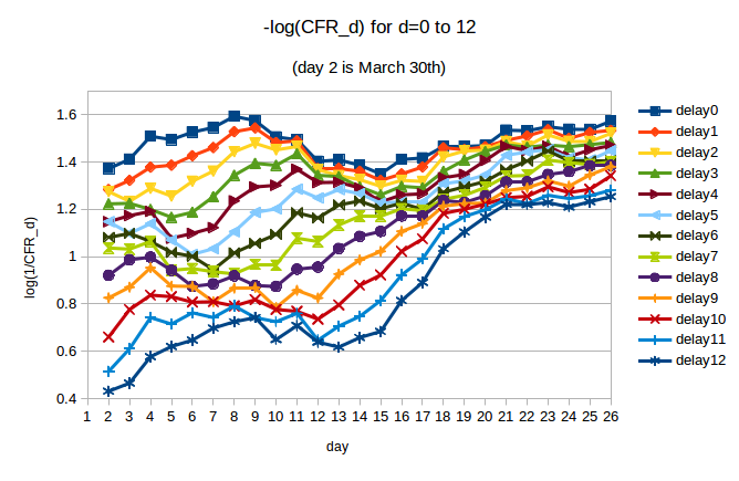
We can try to do this by looking at the variation in CFR_d during the early period for different values of C-F delay d. In the next figure we plot -log(CFR_d) for d = 0 … 12. We are interested in the period from March 30th (day 2 in the plot) to April 10th (day 13 in the plot). If CFR_d is approximately constant over this period, then we can say that fatalities were well-predicted by cases d days earlier. We note, by eye, that the curves are flatter for some values of d than others.
We use regression to quantify the trend in CFR_d over the period of interest. For d from 0 to 12, we compute the slope of the line of best fit through the values of -log(CFR_d) over the period from day 2 (March 30th) to day 13 (April 10th). The slopes, along with 95% CIs, are plotted below:
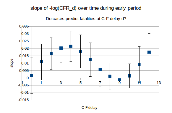
We see that for d = 0, 1, 7, 8, 9,10 and 11, the 95% CIs include 0. The calculated slope is smallest in magnitude for d = 8, 9 and 10, and so is the standard error on this slope. This provides some evidence that cases predict deaths with greater accuracy (during the early period) if we use a longer C-F delay. This would imply that it is the higher end figures for prevalence and fatality undercounting in which we should place greater trust.
Effects of various assumptions on the estimates. The assumptions that case detection and C-F delay remained constant after April 10th are open to question. Test positivity remained fairly constant through April, but began to rise in mid-May and has continued to rise since, which could mean that case detection decreased subsequently. Further, it is plausible that C-F delay could fall as time progresses, as a smaller and smaller proportion of cases are identified through contact tracing as compared to symptomatic cases.
A drop in either case detection or C-F delay over time would lead to higher values for both prevalence and fatalities than those presented here. It is easy to see why a drop in case detection leads to higher estimates of infection – and hence fatality: the detected cases are a diminishing fraction of the total. This implies that the detected fatalities are again a diminishing fraction of the total. On the other hand, a drop in C-F delay means that cases are reflecting infection with a greater delay; working backwards, this increases estimates of infection and, once again, of fatalities.
Thus the main sources of possible error push values for infections and fatalities upwards.
Some final estimates. Let’s finish with some estimates. If I were asked to guess at prevalence and fatality undercounting based on the techniques above, I would guess at between 15 and 25 million infections nationwide currently – at the end of June (i.e., 1% to 2% prevalence); and fatalities to be between 2 and 4 times those recorded (i.e., at the end of June 35,000 to 70,000 COVID-19 fatalities have occurred). Of course, data could become available which would prove these estimates wildly wrong. But of one thing I am fairly certain: if prevalence is much higher than in these estimates, then so too will be the missing fatalities.
Addendum (06/07/2020): What similar analysis tells us about Germany’s COVID-19 epidemic
I decided to add into this document some analysis of Germany’s data in the same vein as the analysis above to provide some comparison with the Indian situation. The methodology is the same: the basic idea is to use early data to estimate C-F delay and see whether we come to the conclusion of underreporting of deaths. The size and number of blocks of data used are the same as in the Indian case.
The early period for Germany was defined as the period upto and including April 5th by which time Germany had recorded 91714 cases and 1342 deaths. Comparing with April 10th for India when there were 7600 COVID-19 cases and 252 recorded COVID-19 deaths it might appear as though we are using more data for Germany; but the difference in numbers reflects the much more rapid progression of the German epidemic, and the higher levels of testing. In particular April 5th was 26 days after Germany’s first recorded COVID-19 fatality, whereas April 10th was 29 days after India’s first recorded COVID-19 fatality.
As we did for India, we look at the variation in CFR_d during the early period for different values of C-F delay d. In the next figure we plot -log(CFR_d) for d = 0 … 12. We are interested in the period from March 25th (day 1 in the plot) to April 5th (day 12 in the plot). If CFR_d is approximately constant over this period, then we can say that fatalities were well-predicted by cases d days earlier.
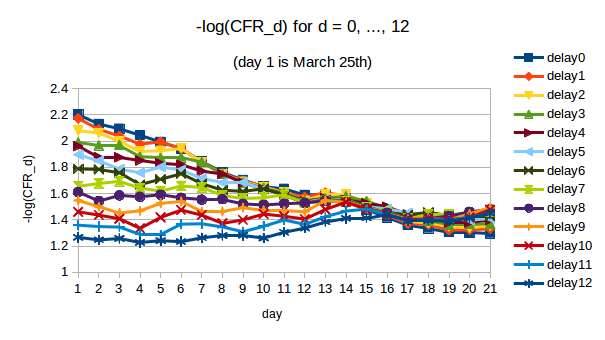
Visually we can spot that some values of d give CFR_d which is approximately constant while others clearly do not. With the larger numbers and better quality data, when we use regression to quantify the trend in CFR_d over the period of interest the results are very clear. For d from 0 to 12, we compute the slope of the line of best fit through the values of -log(CFR_d) over the period from day 1 (March 25th) to day 12 (April 5th). The slopes, along with 95% CIs, are plotted below:
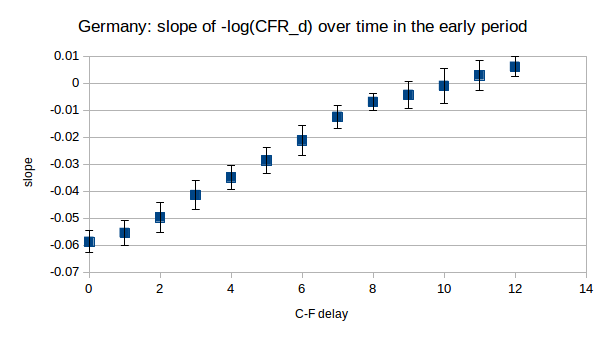
We see that only for d = 9, 10 and 11 do the 95% CIs on the slope include 0. These are the values for which we cannot reject the hypothesis that CFR_d was constant over this period. Moreover, there is a clear trend in the slopes (they decrease as d increases as we would expect), which allows us to say with some confidence that the “true” early C-F delay lies somewhere around these values.
So, we plot the estimates of Germany’s “missing” COVID-19 fatalities for d = 9, …, 12.
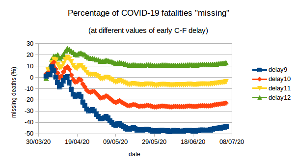
For d = 9 and 10 we find that the “missing deaths” are negative(!), namely that recorded deaths are greater than predicted deaths by about 44% (d=9) and 23% (d=10). This underprediction of deaths is even more marked at shorter delays (not plotted). For d = 12 we find about 13% missing deaths. However, the regression analysis suggested that d=12 was not a credible estimate for the early C-F delay. For d=11 we find small negative “missing deaths” – namely recorded deaths are about 4% more than predicted.
What can we conclude? There is no signature of increasing “missed” deaths in the German data as the epidemic surged. With a C-F delay of around 11 days – a plausible value for the true C-F delay from regession analysis – the early delayed CFR predicts subsequent deaths quite accurately, all the way upto the present. Incidentally early CFR_11 for Germany was 4.5%, namely early analysis with C-F delay of 11 days would already have suggested that about 4.5% of Germany’s identified COVID-19 infections would result in death, as has currently been observed.
In some ways, Germany’s epidemic presents an opposite picture to India’s. There are no unexplained or surprising changes in fatality during the course of the epidemic. On the other hand, in the Indian data recorded fatalities are significantly below expected fatalities for a wide range of values of early C-F delay, including implausibly short delays. Even for d=0 – terribly late case detection inconsistent with contact tracing – we get about 9% of deaths missing today.